The rule cursor and central slide can be positioned using a mouse. Fine adjustment can be achieved using the keyboard left and right arrow buttons. The keyboard keys move the cursor or slide depending upon which had last been clicked or adjusted.
The left hand display below the rule (“A on B” etc) shows the slide position. The central display shows the cursor position over each of the slide scales.
Why is the cursor window a bit yellow? To find out, check my blog where some of the design decisions that went into constructing this rule are described. Thats also a good place to comment if you come across any gross bugs (bugs are likely of course but so are edge cases that maybe should be treated kindly).
The Calculator
You can try using the virtual calculator just like a normal one although the choice of functions and the absence of plus and minus buttons might be a little eccentric. Please remember though that calculations performed on a slide rule will not always be as accurate as those performed on an electronic calculator. Results can and will differ.
You can enter values using the “buttons” or from your keyboard (including the numeric keypad if “Num Lock” is set. The sum is executed by the virtual slide rule and the result read back from the slide rule. The division function is executed in two stages with a 1.5 second delay between them. An experienced slide rule user would probably skip the second stage as the result can be read from the end of the slider.
You can calculate the tangent of angles (in degrees) between 6° and 84°. The S (sine) scale is also used to calculate cosines – both in the range 1° to 90°.
Background
I was looking through some bits and bobs that came from a drawer in my Father’s house when it was being cleared for sale. One of the items was a slide rule and it was found alongside the early “Sinclair Executive” calculator that replaced it. It is small (nominally 6" probably) and pretty similar to the one I remember buying with my first student grant money in the very late 1960s when they were still pretty much the state of the art for calculators. Around that time though, I did come into contact with an electronic Anita calculator but they were staggeringly expensive and you could hardly slip one in your pocket or even carry one very far.
The Sinclair Executive calculator came out in 1972 and cost £79.95 (over £1000 in 2020 money) and I probably paid £5 or £6 for the slide rule three or four years before that (still an appreciable cost that needed some internal debate to justify).
The slide rule was invented sometime between 1620 and 1630 with new functions developed and added over time until the device became the tool of choice for the developing field of engineering.
How do they work? It is pretty easy to see how two rulers could be used to do simple addition and subtraction. We can try adding 3 and 8.
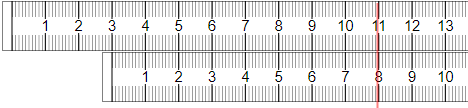
We position the start on the lower ruler’s scale at one of the two values (in this case 3) and read off the sum of 3 and 8 on the scale of the upper ruler (see the red line). It should also be obvious that the same positioning could be used to calculate 11 minus 8 or any other pair of values on the two ruler scales.
Now such a simple mechanical device for adding two numbers together would not be terribly useful even if they were decimal fractions such as 3.4 and 8.7
which would be easy to do with the rulers shown above. However being able to multiply (say) 1.65 by 3.45 would be more challenging mental arithmetic for most.
When I was at school, we used logarithms for such calculations.
The logarithm (base 10) of a number is the number expressed as a power of 10.
1.65 = 100.2175 so log(1.65) = 0.2175
3.45 = 100.5378 so log(3.45) = 0.5378
0.5378 + 0.2175 = 0.7553 (sum the logs)
100.7553 = 5.6925 which is the product of 1.65 and 3.45.
Thus simple addition can be used to multiply two decimal fractions expressed as logarithms.
Fortunately, when I was at school, we did not need to calculate these powers of 10 – we were issued with books of tables for looking them up. The tables included a host of trigonometric tables as well as the vital “antilogarithms” needed to establish that 100.7553 was 5.69 (which was about as accurate as the ones I had could get.
If instead of having pages of tables we were to draw a logarithmic scale on a pair or rulers instead of the linear scale illustrated above we could use them to multiply two values by adding the logs. Indeed we could also do division by subtracting one logarithmic scale position from another. So, what does a logarithmic scale look like in action?
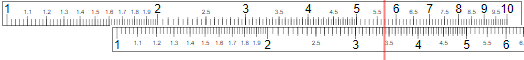
You will notice that as the values increase (from 1 to 10 in this instance) the distance between the log of those values decreases. You can probably also see that two rules with logarithmic scales can be used to make our calculation (1.65 x 3.45). Slide rules were fast and accurate enough for most purposes.
Why does the log scale start at 1? Well ten to the power of zero is 1 and zero is a good place to start. In fact any number to the power of zero is 1.